University Physics
Electromagnetics Lab
Lab 3 ResistorñCapacitor Circuits
In this lab, we shall investigate RESISTOR-CAPACITOR circuits, or as they are commonly
known, ìRCî circuits. Unlike typical situations involving batteries and networks of resistors,
in which steady-state behavior is quickly realized, RC circuits evince more readily
observable exponentially-limited growth, or decay, of salient properties.
In the course of performing this experiment, we shall reinforce
- proper use of electrical meters,
- notions of direct and indirect measurement,
- proper employment of semi-log graph paper,
- use of experiment to corroborate or falsify theory, and
- error analysis.
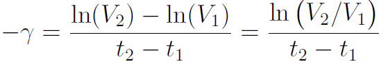
GRAND IDEA: By careful analysis, we will measure the charging and discharging time
constant(s) [OR the DECAY RATE(S)] governing particular RC circuits. We will also infer the
actual capacitance of the system.
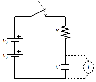
CHARGING
The electric potential difference [VOLTAGE] across a charging capacitor is expected
to have the following time-dependence:
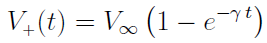
where  is the asymptotic (long time) value of the voltage, and
 is the charging
and discharging rate characteristic of the system.
is the charging
and discharging rate characteristic of the system.
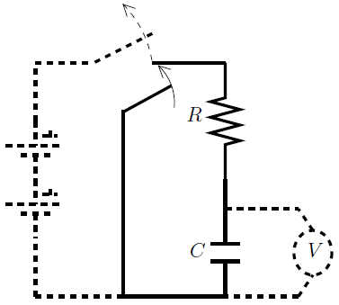
DIS-CHARGING
The predicted form of the electric potential across a discharging capacitor is:
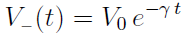
where Vo in this case is the starting (t = 0) value of the potential.
According to the theory describing the dynamical behavior of RC-circuits,
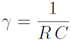
where R, the resistance, is in Ohms [W],
and C, the capacitance, is in Farads [ F ].
Our tools for this experiment include: [LARGE-valued] capacitors and resistors, a circuit
breadboard, wires, batteries, meters, and a stopwatch.
WARNING: the capacitors that we use are oriented, that is, they are engineered, so that
positive charge accrues to one plate only. The orientation is indicated by a dark arrow
residing in a light-grey band on the barrel of the capacitor. The positive terminal of
the battery is connected on the POSITIVE side, the base of the arrow, while the negative
terminal is connected to the NEGATIVE capacitor lead, at the arrowhead.
Reflect upon your observations.
Q: Does the voltage across the capacitor experience exponentially-limited
growth on charging and exponential decay on discharging, as predicted?
Q: Are the charging and discharging rate constants equal?
Combine the two decay rates to obtain a single range for
, and from this and
the measured value of the resistance, infer the capacitance.
CAVEAT: Stated values of capacitance are usually about 25% precise.